data mining, grab your helmet.

Last fall I took a data mining course and learned a basic element of problem solving, building a mathematical model out of data. It’s not too hard of a task, it can be accomplished with one key in Matlab, but the lack of basic tutorials on principle component analysis are what drove me to etch out this little space on the internets. I’m by no means an expert on PCA, I simply want to show you how to use it to build a model in Matlab… and as long as I’m doing that I might at well show you the other way I made other models.

While I provide you with the source code for my project I hope this tutorial is helpful without having to dig through those files. Feel free to provide feedback positive or negative.

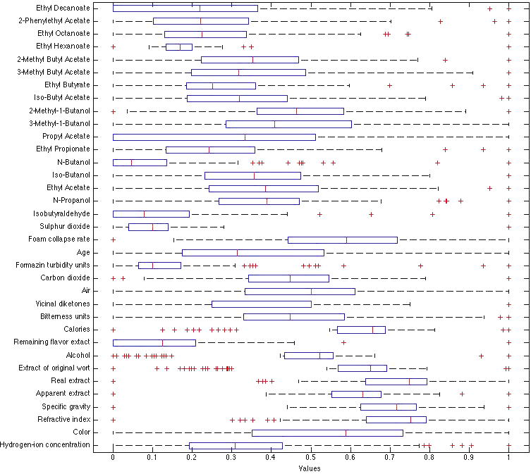
This plot is really unnecessary. This is just a normalized boxplot of my input variables. I’m doing this to show you I’m working with real data and to remind you to normalize your input variables.

Linear Regression

Linear regression is a way to develop a best fit solution to an over constrained set of equations. Performing least squares regression, a type of regression that minimizes the error, is such a common problem in Matlab that its function has been assigned to the backslash operator. Calculating a least squares regression model can be performed like so:

X = [ones([size(training_data,1),1]) training_data(:,inputs)];
a = X \ training_data(:,result_column);
X = [ones([size(actual_data,1),1]) actual_data(:,inputs)];
Prediction = X*a;

Where inputs could be a single input column or an array of inputs. Adding inputs to the model increases its fit to the training data while increasing complexity. It’s important to find a balance between the number of variables used in regression and the quality of fit. Fortunately a few statistical criterion have been established to alleviate this dilemma. The Bayesian and Akaike information criterion are tools for model selection.

Here is a list of my inputs arranged according to their correlation with the training data:

Column,  Correlation,    P Value,   Description:
  11,      -0.2934,    0.0047,      BU: Bitterness units. 
  27,       0.2760,    0.0080,      2-Methyl-1-Butanol
  15,      -0.2380,    0.0230,      FTU: Formazin turbidity units.
  14,      -0.2089,    0.0468,      C02: Carbon dioxide.
  20,      -0.2018,    0.0550,      N-Propanol
  33,       0.1939,    0.0655,      Ethyl Octanoate
  35,       0.1867,    0.0763,      Ethyl Decanoate
  21,       0.1617,    0.1256,      Ethyl Acetate

Here is a list of the MaxError, RSS, BIC, and AIC as a function of the number of inputs in my model. The eight numbers correspond to the eight most highly correlated inputs in my data. The first number in each column corresponds to a model with only one input, the second corresponds to a model with two inputs…

MaxError:
0.970, 0.805, 0.759, 0.764, 0.764, 0.707, 0.719, 0.729
Residual sum of squares:
9.366, 8.543, 8.279, 7.967, 7.967, 7.606, 7.405, 7.400
Bayesian information criterion:
6.748, 11.16, 15.64, 20.11, 24.62, 29.09, 33.57, 38.08
Akaike information criterion:
49.39, 48.19, 49.14, 49.88, 51.88, 52.41, 53.58, 55.56

While the Bayesian information criterion (BIC) suggests I build my linear regression model with only one input, the bitterness units, BIC is well known for over penalizing the number of variables used in a model. The Akaike information criterion suggests I use a model with two inputs, bitterness units and 2-Methyl-1-Butanol; I agree. Adding additional inputs to this model would improve its fit to the training data but not necessarily other sets of data. As such, my linear regression model is based upon the two inputs most strongly correlated to the output of my training data, which lie in column 11 and 27:

a = [ 5.9215; -0.0496; 0.0367]
y = 5.9215 - 0.0496*C11 + 0.0367*C27;

L1Linear Regression

I didn’t use L1Linear Regression in this course, but it’s another modeling system I can use to compare with my results. There’s a great explanation of how to perform L1 regression in Matlab here: Matlab Data Mining

X = [ones([size(training_data,1),1]) training_data(:,inputs)];
a = L1LinearRegression(X, training_data(:,end))
X = [ones([size(actual_data,1),1]) actual_data(:,inputs)];
Prediction = X*a;

MaxError:
0.945, 0.829, 0.741, 0.754, 0.753, 0.720, 0.731, 0.728
Residual sum of squares:
9.431, 8.742, 8.435, 8.082, 8.086, 7.822, 7.662, 7.684
Bayesian information criterion:
6.754, 11.18, 15.66, 20.13, 24.64, 29.12, 33.61, 38.12
Akaike information criterion:
49.63, 48.97, 49.76, 50.35, 52.36, 53.30, 54.64, 56.73

The results are quite similar to that of standard linear regression. I’m really just putting it here for perspective… the L1LinearRegression model is:

a = [ 5.6242; -0.0267; 0.0345]
y = 5.6242 - 0.0267*C11 + 0.0345*C27;

Principle Component Analysis

Amazing! Someone actually read this far. As PCA was the impetus of this little article, I’m embarrassed to say that I’m still working on my understanding PCA. I really don’t want to lead anyone astray. Once I make sure I did everything properly I’ll finish this up. Until then, you can view my working directory here.

Finally the last technique I used was principle component analysis. PCA is best defined as “an orthogonal linear transformation that transforms the data to a new coordinate system such that the greatest variance by any projection of the data comes to lie on the first coordinate.”

The Matlab function princomp is helpful for PCA as it automatically computes the principle component coefficients, the scores (the data translated to the new coordinate system), and the variance of each principle component. Like the other models, I recorded the accuracy of each PC model as a function of the number of principle components used. While there is a negative linear relationship between the number of PC used and the RSS, that slope is shallow compared to that of the regressions.